Branin Function Example
The Branin function is a 2-dimensional continuous benchmark function commonly used to test optimization algorithms. It has three global minima and multiple local minima, making it ideal for demonstrating iterative optimization workflows like AMLRO.
Function Domain
Variable |
Bounds |
|---|---|
x₁ |
[-5, 10] |
x₂ |
[0, 15] |
Global Minima
(-π, 12.275)
(π, 2.275)
(9.42478, 2.475)
All minima have a function value of approximately 0.3979. since we going to use coaser grid Minima ~0.40
Purpose
Demonstrate AMLRO workflow with a computational benchmark.
Show reaction space generation, training set creation, and active learning prediction.
Click the badge below to open this notebook in Google Colab:
![]()
from amlro.optimizer import *
from amlro.generate_reaction_conditions import *
from amlro.generate_training_data import *
import random
import matplotlib.pyplot as plt
import pandas as pd
config = {
            "continuous": {
                "bounds": [[-5, 10], [0, 15]], #
                "resolutions": [0.1, 0.1],
                "feature_names": ["f1", "f2"],
            },
            "categorical": {
                "feature_names": [],
                "values": []
            },
            "objectives": ['fx'],
            "directions": ['min'],

        }
exp_dir = 'Branin_test'
sampling = 'sobol'
training_size = 20
regresor_model = 'gb'
Step 1: Generate Reaction Space
Reaction space generation serves two purposes:
Construct the full combinatorial reaction space based on user-defined continuous and categorical parameters.
Select an initial subset of reactions for training using a chosen sampling strategy.
Please run the following cell/code line.
get_reaction_scope(config=config, sampling=sampling, training_size=training_size, write_files=True, exp_dir=exp_dir)
d:\amlro\venv\lib\site-packages\scipy\stats\_qmc.py:763: UserWarning: The balance properties of Sobol' points require n to be a power of 2.
  sample = self._random(n, workers=workers)
(         f1    f2
 0      -5.0   0.0
 1      -5.0   0.1
 2      -5.0   0.2
 3      -5.0   0.3
 4      -5.0   0.4
 ...     ...   ...
 22796  10.0  14.6
 22797  10.0  14.7
 22798  10.0  14.8
 22799  10.0  14.9
 22800  10.0  15.0

 [22801 rows x 2 columns],
          f1    f2
 0      -5.0   0.0
 1      -5.0   0.1
 2      -5.0   0.2
 3      -5.0   0.3
 4      -5.0   0.4
 ...     ...   ...
 22796  10.0  14.6
 22797  10.0  14.7
 22798  10.0  14.8
 22799  10.0  14.9
 22800  10.0  15.0

 [22801 rows x 2 columns],
      f1    f2
 0  -5.0   0.0
 1   2.5   7.5
 2   6.3   3.7
 3  -1.2  11.2
 4   0.6   5.6
 5   8.1  13.1
 6   4.4   1.9
 7  -3.1   9.4
 8  -2.2   4.7
 9   5.3  12.2
 10  9.1   0.9
 11  1.6   8.4
 12 -0.3   2.8
 13  7.2  10.3
 14  3.4   6.6
 15 -4.1  14.1
 16 -3.6   7.0
 17  3.9  14.5
 18  7.7   3.3
 19  0.2  10.8)
Define Branin objective function
The Branin function is defined as:
[ f(x_1, x_2) = a (x_2 - b x_1^2 + c x_1 - r)^2 + s (1 - t) \cos(x_1) + s ]
with typical constants:
(a = 1)
(b = 5.1 / (4 \pi^2))
(c = 5 / \pi)
(r = 6)
(s = 10)
(t = 1 / (8 \pi))
def branin(x):

    x1, x2 = np.array(x)

    a = 1.0
    b = 5.1 / (4.0 * np.pi**2)
    c = 5.0 / np.pi
    r = 6.0
    s = 10.0
    t = 1.0 / (8.0 * np.pi)


    return a * (x2 - b * x1**2 + c * x1 - r)**2 + s * (1 - t) * np.cos(x1) + s
Step 2: Initial Training Data (closed-loop)
This step collects objective results for the initial parameter combinations.
objective values are collected by calling branin objective function each iteration.
parameters = []
objectives = []

for i in range(training_size):

    parameters = generate_training_data(exp_dir=exp_dir,config=config,parameters=parameters, obj_values=objectives)
    print(parameters)
    objectives = [branin(parameters)] # Branin objective function

generate_training_data(exp_dir=exp_dir,config=config,parameters=parameters, obj_values=objectives,termination=True)
[-5.0, 0.0]
writing data to training dataset files...
[2.5, 7.5]
writing data to training dataset files...
[6.3, 3.7]
writing data to training dataset files...
[-1.2, 11.2]
writing data to training dataset files...
[0.6, 5.6]
writing data to training dataset files...
[8.1, 13.1]
writing data to training dataset files...
[4.4, 1.9]
writing data to training dataset files...
[-3.1, 9.4]
writing data to training dataset files...
[-2.2, 4.7]
writing data to training dataset files...
[5.3, 12.2]
writing data to training dataset files...
[9.1, 0.9]
writing data to training dataset files...
[1.6, 8.4]
writing data to training dataset files...
[-0.3, 2.8]
writing data to training dataset files...
[7.2, 10.3]
writing data to training dataset files...
[3.4, 6.6]
writing data to training dataset files...
[-4.1, 14.1]
writing data to training dataset files...
[-3.6, 7.0]
writing data to training dataset files...
[3.9, 14.5]
writing data to training dataset files...
[7.7, 3.3]
writing data to training dataset files...
[0.2, 10.8]
writing data to training dataset files...
Training set generation completed..
Step 3: Active Learning Optimization Loop
This step uses the initial dataset to train a model and predict the next batch of parameters for minimizing the objective function
%%capture
parameters = []
objectives = []
for i in range(1):
    parameters = get_optimized_parameters(exp_dir=exp_dir,config=config, parameters_list=parameters,objectives_list=objectives, batch_size=1, model= regresor_model)
    print(parameters)
    #objectives = [[branin(parameters[0])],[branin(parameters[1])]] #if you use batch size = 2 You need to call branin fucntion two time for each parameter set.
    objectives = [[branin(parameters[0])]] #user input

get_optimized_parameters(exp_dir=exp_dir,config=config, parameters_list=parameters,objectives_list=objectives, batch_size=1, termination=True)
df = pd.read_csv(f'{exp_dir}/reactions_data.csv')
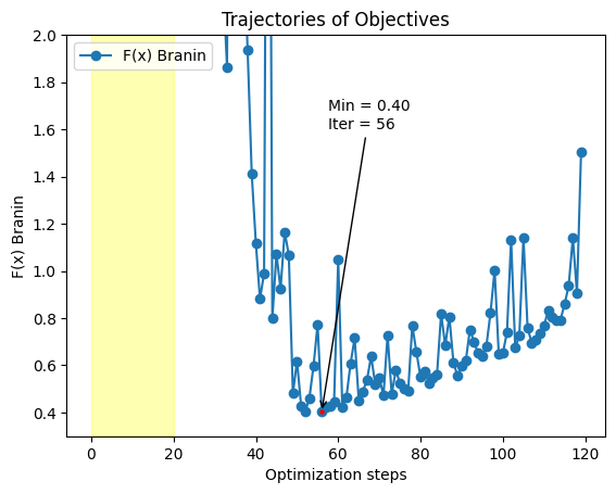
plt.plot(df['fx'],marker='o', label="F(x) Branin")
plt.axvspan(0, training_size, color='yellow', alpha=0.3)
min_idx = df['fx'].idxmin()
min_val = df['fx'].min()
plt.scatter(min_idx, min_val, color='red', s=5, zorder=5)
plt.annotate(
    f"Min = {min_val:.2f}\nIter = {min_idx}",
    xy=(min_idx, min_val),
    xytext=(min_idx + 1.5, min_val + 1.2),
    arrowprops=dict(facecolor='black', arrowstyle='->'),
)
plt.legend(loc='upper left')
plt.xlabel('Optimization steps')
plt.ylabel('F(x) Branin')
plt.ylim(0.30,2)
plt.title('Trajectories of Objectives')
Text(0.5, 1.0, 'Trajectories of Objectives')
x1 = np.linspace(-5, 10, 100)
x2 = np.linspace(0, 15, 100)
X1, X2 = np.meshgrid(x1, x2)
Z = branin([X1, X2])
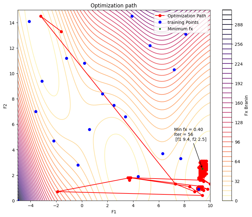
plt.figure(figsize=(10, 8))
plt.contour(X1, X2, Z, levels=50, cmap='magma_r')
plt.colorbar(label='Fx Branin')
plt.plot(df['f1'][training_size:], df['f2'][training_size:], 'o-', color='red', markersize=6, label='Optimization Path')
plt.plot(df['f1'][:training_size], df['f2'][:training_size], 'o', color='blue', markersize=6, label='training Points')
min_idx = df['fx'].idxmin()
min_val = df['fx'].min()
min_f1 = df.loc[min_idx, 'f1']
min_f2 = df.loc[min_idx, 'f2']
# Highlight minimum point
plt.scatter(min_f1, min_f2, color='green', s=10, zorder=5, label='Minimum fx')
# Annotate with value and iteration
plt.annotate(
f"Min fx = {min_val:.2f}\nIter = {min_idx} \n [f1 {min_f1}, f2 {min_f2}]",
xy=(min_f1, min_f2),
xytext=(min_f1 - 2.2, min_f2 + 2.2), # offset for visibility
arrowprops=dict(facecolor='black', arrowstyle='->'),
)
plt.xlabel('F1')
plt.ylabel('F2')
plt.legend()
plt.title('Optimization path')
Text(0.5, 1.0, 'Optimization path')